
| e1 | e2 | e3 | |
|---|---|---|---|
| h1 | 0.00 | 0.75 | 0.75 |
| h2 | 0.75 | 0.00 | 1.50 |
| h3 | 0.75 | 1.50 | 0.00 |
MEAPS: Modelling commuter flows 1
1 Translation by Scotia Hille
The gravity model used to distribute journeys between an origin and a destination poorly represents the influence of distance on choices. Drawing on the ‘intervening opportunities’ model of Stouffer (1940) and the radiative model of Simini, González, Maritan, & Barabási (2012), we construct an ergodic model of absorption with priority and saturation (MEAPS) that makes it possible to construct these choices on clear and flexible microscopic foundations. The model accommodates different formulations of stochastic processes that allow fundamental parameters to be estimated and interpreted. We validate the theoretical model on synthetic data, then in two associated documents (Parodi & Timbeau, 2024b, 2024a) We propose an estimate of MEAPS and a detailed comparison with the gravity model and its most common variants. We then use this modelling to construct a high-resolution map of CO2 emissions in La Rochelle.
5435 words.
5435 words.
1 Tobler does not imply gravity
In the analysis of spatial phenomena, distance plays an important role. This is sometimes referred to as Tobler’s principle:
Everything is related, but things that are close are more related than things that are far away.
If we take the example of the geographical matching of jobs and residents, proximity to the workplace is a critical factor, even if other factors come into play in the choice of a job: salary, skills, etc. The role of distance in job choice is generally assessed using a gravity model. Few alternatives have been studied in the literature, and the gravity model has become standard: an analytic tool that need not be brought into question, allowing the focus to rest on other factors.
However, when we looked at the mobility of daily life on a fine spatial scale – the 200 metre square – we came up against the limitations of the gravity model, particularly when it came to deciding on scenarios for the geographic redistribution of jobs. These limitations stem from the fact that the gravity model reduces Tobler’s principle to a homogeneous measure of distance. Within the gravity model, it is possible to significantly improve our understanding of a given territory’s spatial dynamics by shifting from an analysis based on distance to one of transport times, calculated according to the different possible modes. Even more precise, it is possible to move to a notion of the generalised cost of a journey, which takes into account different aspects of that journey (its monetary cost, comfort, reliability, etc.). However, these improvements to the ‘metric’ – undeniable though they are – merely change the input to the gravity model, without questioning it. Yet, this model suffers from a more fundamental flaw: it overlooks what makes space unique by trying to reduce it to a one-dimensional variable; it overlooks the fact that space is inhabited and that each place is also defined by its neighbourhood.
For example, the gravity model treats dense urban environments and rural areas in the same way. You’d think, for example, that a half-hour car journey would be just as hard for a “gilet-jaune” (“yellow vests”, referring to rural or suburban residents) as it is for a Parisian. However, this is clearly not the case: people living in rural areas make a virtue of necessity and even end up appreciating these long daily journeys, whereas people living in highly urbanised areas consider alternatives because they have a wider range of options to satisfy their demands. The flaw in the gravity model is thus not a simple matter of subjective relationships to journey times. More fundamentally, the fault lies in the fact that this model does not see space; it does not see what the territory offers; it does not see that in urban areas the array of opportunities (of jobs, services, etc.) is more compact and that this changes the way relative distances and relative costs are treated. The consequence of this blindness is that the supply in the area is treated as if it were homogeneous. Suppose, for example, that the public authorities want to create an industrial estate offering new jobs. The gravity model would lead us to believe that residents of rural areas, because they are so scattered, are usually too far from the new employment zone to be interested: in the trade-off between the usefulness of the job and the cost of the journey, the latter quickly becomes so high that it seems preferable to give up the job. However, the real trade-off is far from being so simplistic because, of course, an individual who cannot find a job nearby will resign himself to travelling further to work than someone who lives near a dynamic economic centre. Distance does not carry the same weight depending on the quantity of opporutnities in the neighbourhood.
Faced with these anomalies linked to the gravity model, we propose to use another analogy: that of a flow of particles passing through a material made up of heterogeneous absorption sites. If someone is looking for a job in an area rich in jobs, the chance of finding one near their point of departure will be high, as is the chance of a particle being rapidly absorbed when it is surrounded by absorbing sites. Conversely, if jobs are not very dense where one lives, the distance one has to travel is likely to be greater, like a particle crossing an area of vacuum. In fact, the chance of being absorbed does not depend directly on the distance to the receiving site; it depends on the number of sites that are crossed before it. Or, to put it another way, it depends on the rank of this site in the ranking of sites from closest to furthest away. This analogy can already be found in Stouffer (1940) and Simini et al. (2012). However, the models they have developed can still be improved, in particular by accounting for the fact that absorption sites can have a limited capacity. The neighbourhood then plays a role both in terms of jobs, which are more or less dense around a given residence location, and also in terms of competitors for jobs, who are themselves more or less dense in that same area.
We therefore propose a model that takes account of absorption and saturation. It is stochastic in nature and, using statistical physics reasoning, we can conjecture that the main predictions are stationary. We have called it the Ergodic Absorption and Saturation Model, or MEAPS for short.
This model also respects the principle that – all other things being equal – what is close plays a more important role than what is far away. But instead of distance, we use rank within classed distances. The difference may seem minor, but it addresses the issue of spatial heterogeneity and the density of the environments crossed. In the gravity model, there always comes a time when, to take yet another example, the school is too far away and it’s no longer “worth” the cost. In the perspective initiated by Stouffer, and applied here, the nearest school, of rank 1, remains useful regardless of how far away it may be, precisely because it is the nearest. The remarkable series of documentaries entitled “Les chemins de l’école” (“Paths to school”) underline perfectly that the nearest school is always worthwhile, even if schoolchildren have to walk several hours to get there.
This analogy allows us to consider the job-matching process as the result of a search procedure that examines opportunities in the order of their proximity. Such a procedure makes it possible to specify behaviours that serve as a reference and as a null hypothesis for examining the data. Marginal amendments to this search procedure could produce a better fit and be interpreted directly. For the time being, we ignore all the other determinants of the match, such as salary, skills required or offered, and sector of activity. We fit a reduced model to the distance argument based on rich data from France’s mobility survey, concerning flows between communes of residence and communes of employment. Under the assumption that all jobs differ only in their location, we achieve a much better fit than the gravity model. More refined data – assuming it exists – could further improve the fit by introducing wage or skill differentials, for example. Nevertheless, taking a more rigorous account of geography seems to us to be an essential first step, since it modifies the quality of the fit by at least an order of magnitude.
The approach is therefore structural: it is a model, even a simple one, that defines the way in which the data can be interpreted. The data without the model means little, the model without the data is mere speculation; thus, following Kant’s injunction, we combine the one with the other to describe reality.
This document describes the construction of the theoretical model. In it we develop our critique of the gravity model section 2 , and develop the analogy of the radiative model section 3. The complete model is not solvable in a closed form. We therefore outline an algorithm for simulating it. In a final section, section 4 we analyse the main properties of the theoretical model on synthetic simulations, i.e. generated from known processes. In the absence of demonstration, this allows us to give credibility to the ergodicity property of the model, which conditions the possibility of simulating it.
In two other papers, we estimate the model on real data and make a detailed comparison with the gravity model and its most common variants (Estimates at La Rochelle). We then use this modelling to discuss the link between density and CO2 (Compact city). We are currently building a high-resolution map of CO2 emissions in La Rochelle using a projection that incorporates frequency and pattern association behaviour for different household categories.
2 Gravity modelling
To model journeys between places of residence and places of employment, analyses typically rely on the 4-step method. (Dios Ortúzar & Willumsen, 2011; Patrick Bonnel, 2001). This method involves first determining the number of journeys originating from a place of residence and, second, the number of journeys arriving in total at a place of work. These make up stage 1: trip generation. The second stage consists of distributing these journeys between each origin-destination pair. This is the distribution stage. The third stage is the modal choice stage, in which an appropriate mode of transport is associated with each journey. Finally, the fourth stage of the model is the one that specifies the journey and provides information about its precise characteristics, such as the route taken or the changes in elevation traversed, which serves particularly to predict traffic and congestion. However, this breakdown into steps is somewhat arbitrary and does not align with best practice for articulating these 4 moments. For example, the number of journeys made depends on the possibilities opened up by geography, which are defined by the precise characteristics of the journeys. Step 4 is therefore necessary to understand step 1, and step 4 requires knowledge of modal choices to be useful for the choices made in step 1. Step 2 is necessary to explore trip possibilities. There are many overlaps between the stages, and the breakdown does not preclude going back and forth between the various stages.
The model we develop here focuses on stage 2, that of the distribution of journeys between the different origin-destination pairs, or residence-jobs. The gravity model is largely dominant in this second stage to take into account the role of distance in the trade-off between different destinations.
In the first part we discuss the shortcomings of the gravity model section 2.1. We then present the intervening opportunities model of Stouffer (1940) and the radiative model of Simini et al. (2012) and Simini, Maritan, & Néda (2013). Both models use job ranking rather than pure distance section 2.2 based on an analogy that is more appropriate to the geographical scales we are considering (municipality, region) than that of gravitation. Finally, in line with these approaches, we develop a model based on the following two ideas:
Individuals make their trade-offs not as a direct function of distance, but as a function of the rank (in the order of distances) of the opportunities available to them. Another way of looking at it is that the number of jobs available in a circle of given radius is a better metric than distance.
Each destination has a limited capacity, so we need to introduce a notion of saturation that forces individuals to look elsewhere. In this way, we establish a basis for respecting the constraints at the margins (every individual has a job, every job is occupied by an individual) and introduce the neighbourhood both at the destination and at the origin.
The final formulation is probabilistic and we analyse some of its properties using synthetic simulations (section 4), showing that we can quickly simulate a state that is independent of the initial conditions.
2.1 The inadequacies of the gravity model
The gravity model develops an analogy with Isaac Newton’s model of universal gravitation, whose successes in physics and mechanics are indisputable. This model is the cornerstone of the path distribution stage (Dios Ortúzar & Willumsen, 2011; Patrick Bonnel, 2001, p. 160; Sen & Smith, 1995). It is also used in other fields, such as international trade and the analysis of epidemics, which we will not discuss here.
The (mistaken) reasons for the success of the gravity model
Formally, the gravity model describes the strength of a relationship between two objects as a function of their respective distance and mass. By analogy, the gravity model consists here of evaluating the number of professional-related trips between two locations by taking as the masses the number of inhabitants at the point of departure and the number of jobs at the point of arrival and, as the denominator, a function of f increasing function of distance2. Thus, if we indicate the starting points by i and the end points by j :
2 The distance can be any metric that distinguishes points in space. The Euclidean distance comes to mind, but the model can also be adapted to take into account distances through transport networks, including journey times to account for different speeds by mode, by type of road used, by time of day, or to compare modes for which distance is of little significance (public transport, because of waiting times and specific lanes). We can also consider a full cost (including both the time and monetary cost of the mode of transport) or a generalised cost including the perceived comfort or safety associated with the mode of transport. Following Koenig (1980), we can use logsum to take into account the variety of solutions for getting to a destination.
T_{i,j} = \frac {N_{hab, i}\times N_{emp, j}} {f(d_{i,j})} \tag{1}
The first gravity models borrowed the function f function from Newtonian physics (f=d^2), but other formulations have since been proposed. For example, the function f=e^{d/\delta}function is used in the discrete choice models proposed by McFadden (McFadden, 1974 ; Ben-Akiva & Lerman, 2018). By replacing distance with the notion of generalised transport cost, this functional form can be linked to a choice model with a random utility model. It is also possible to adjust more complex functional forms by adding parameters. The gravity model can thus more or less reproduce the distribution of distances observed in mobility surveys.
Wilson (1967) proposed a reasoning based on entropy minimisation to provide a theoretical basis for equation 1. He identifies the reference state as that which is most frequent in a random distribution of choices. Wilson (1967) then shows that, given the function f , equation 1 in fact has the proposed form, which is the product of inhabitants and jobs that must be in the numerator (and not a power of one or the other, for example). Still, this does not provide a theoretical backing for the functional form of f. The parallel with physics is easy to draw: interaction defines the role of distance, and maximisation of entropy allows us to deduce that the macroscopic equation depends on the aggregate masses, but does not allow us to say anything more about the nature of the interaction.
As Simini et al. (2012) notes, the theoretical and empirical foundations of the f function are weak at best. The multiplication of parameters to improve the fit often has no theoretical justification. In fact, it is often impossible to give any meaning to the estimated parameters, which renders the adjustment exercise opaque. The asymptotic behaviours also highlight inconsistencies: for example, because the model is such that the number of jobs at the point of arrival tends towards infinity, it predicts an infinite number of journeys, even though the number of residents at the point of departure is limited! The gravity model can also be criticized for its deterministic nature, which inhibits it from explaining the statistical fluctuations in the number of predicted journeys, as well as the likelihood of different empirical cases.
Nevertheless, the strongest criticism of the gravity model comes from its fundamental properties and the conclusions that can be drawn from them. The number of journeys between an origin (residence) and a destination (employment) is based on a simple trade-off between distance and the number of residents or jobs. Once again, the behaviour of the model at the limits is perplexing: a single job at the origin should be infinitely preferred to a very large number of jobs a little further away. This is entirely unrealistic, and we can already estimate that distance does not play such a direct role in mobility behaviour. We can also see that, in the gravity model, the relative weight of a quasi-central job in relation to the “masses” of distant jobs would vary widely depending on how close it is to the origin, in an unrealistic manner.
As indicated by Stouffer (1940) , it is perhaps not so much the distance to jobs that is decisive as the rank of these jobs in the order of distances. In the gravity model, there is a big difference between the case where the second nearest job is 500 m away and the case where it is 1 km away. If we apply the Newtonian model, we would have to believe, for example, that the attractiveness of the latter job is divided by 4. Yet, who could believe that a 500 m difference would be such a significant factor in a job search? The attractiveness of the job depends above all on the fact that it is the second job available close to home. Empirically, there is little doubt that the gravity model performs poorly: it fails to explain why, when the density of jobs is low around a resident, he or she will envisage longer journeys to reach areas with a high density of jobs; yet this is a very common observation that should be reflected in adequate modelling.
Simini et al. (2012) give a few examples for the United States of the difficulty of the gravity model in reproducing observed behaviour by outlining a few regularities. Clearly, the gravity model only predicts nearby destinations and completely ignores distant destinations. It seems impossible for the functional form f(d_{ij}) to empirically account for both the number of short journeys and the number of long-distance journeys with a model that functions across different spatial regions, given that densities are distributed differently.
There are relatively few publications that systematically compare the gravity model with other formulations that respect Tobler’s first law. Heanue & Pyers (1966) is one of the first attempts of this kind. Recent work by (Commenges, 2016; Floch & Sillard, 2019; Lenormand, Bassolas, & Ramasco, 2016) confirm what Masucci, Serras, Johansson, & Batty (2013) concluded after the initial publication of the radiative model: that the extended gravity model has better explanatory power regarding to inter-urban mobility flows, a constant which holds for various zones considered across several countries. The usual extension of the gravity model is to write, where c, \alpha, \beta and \delta are positive parameters:
T_{i,j} = c \frac {N_{hab, i}^\alpha \times N_{emp, j}^\beta} {d_{i,j}^\delta} \tag{2}
Estimated parameters \alpha and \beta are usually less than 1, which relates to a problem raised by Simini et al. (2013): in this form the gravity model is non-divisible. If we consider an area in which there are workers (origin) or jobs (destination) and we decide to separate it into two distinct areas 1 and 2, as close to each other as possible, the flows T_1 and T_2 predicted by the estimated form of equation 2 are not the sum of the flow that would be obtained from the two zones combined. This separation into sub-areas might be performed to modify the spatial unit of aggregation (Modifiable Areal Unit Problem) or to identify sub-populations (e.g. by sector, by household category) within the initial zone. This more detailed description can be achieved with different flow behaviours (which justify the division), but in the limited case where these populations cannot be distinguished, there is no reason to expect different behaviours.
This property of separability at both origin and destination is verified, however, for the radiative model. As Simini et al. (2013) suggest, the parameters \alpha and \beta of the gravity model can be explained through the radiative model (see below). These parameters summarise the additional spatial information, and depend on the joint spatial distribution of masses at origins and destinations. However, they are highly dependent on the spatial structure, the unit division and the sub-perimeters considered. In this sense, we return to Fotheringham (1983)’s analysis that the gravity model lacks essential spatial information about neighbourhoods.
The problem of constraint at the margins
The gravity model can be made even more complex to fit the data better than it spontaneously does. It then loses a clear link with the theoretical reflections linking it to the maximisation of entropy. (Wilson, 1967) or the discrete choice model. The adjustment of the model becomes a dummy exercise which does not inspire great confidence, particularly in the analysis of the scenarios modelled. The exercise consists of adding a “normalisation” step by incorporating corrective coefficients in the rows and columns of the origin-destination matrix, which amounts to adding fixed effects to each of the departure and arrival points. The formulation of the gravity model is then modified as follows:
T_{i,j} = a_i \times b_j \times \frac {N_{hab, i}^\alpha \times N_{emp, j}^\beta} {f(d_{i,j})} \tag{3}
Determining the coefficients a_i and b_j coefficients poses a number of problems. These coefficients must make it possible to respect the constraints at the margins: the sum of jobs for a row of residents must be equal to the number of residents employed in the zone and the sum of residents employed at a place of employment must, in column form, be equal to the number of jobs at that place. For a_i (in noting that \Sigma_j T_{ij} = N_{hab,i} and \Sigma_i T_{ij} = N_{emp,j} :
\begin{aligned} a_i &{}= \frac {\Sigma_j T_{i,j}} {\Sigma_j \frac {b_j \times N_{hab, i}^\alpha \times N_{emp, j}^\beta}{f(d_{i,j})}} \ &{}= \frac{N_{hab}^{1-\alpha}} {\Sigma_j \frac{ b_j \times N_{emp,j}^\beta}{f(d_{i,j})}} \end{aligned} \tag{4}
\Sigma_j T_{i,j} is generally observed directly or estimated during the generation stage of 4-stage approaches. It is the number of departures from the i point and is proportional to the number of working people residing in i. Likewise, we can produce for b_j an expression symmetrical to that of a_i , involving \Sigma_i T_{i,j} which is also observed or estimated beforehand. This is the number of journeys converging on the arrival point j which is proportional to the number of jobs in j.
\begin{aligned} b_j &{}= \frac {\Sigma_i T_{i,j}} {\Sigma_i \frac {a_i \times N_{hab, i}^\alpha \times N_{emp, j}^\beta} {f(d_{i,j})}} \ &{}= \frac{N_{emp, j}^{1-\beta}}{\Sigma_i \frac{a_i \times N_{hab,i}^{\alpha}}{f(d_{i,j})}} \end{aligned} \tag{5}
The value of a_i for a given i depends on the evaluation of all the b_j and conversely the evaluation of each b_j depends on that of all the a_i. We can estimate these coefficients by successive iterations and thus hope to reach a fixed point, eventually unique to a close multiplicative constant. Algorithmic solutions have therefore been proposed in the main textbooks. The application of such algorithms (such as Furness’ Dios Ortúzar & Willumsen (2011), p. 192) modifies the result proposed by the expression of the equation 2 gravity model, at the risk of diverging from its logic and initial justifications. Indeed, the a_i and b_j are modifiers of the masses of workers and jobs. To make the gravity model work, you therefore have to ‘cheat’ on the masses. Furthermore, the multiplicity of solutions and the choice made by the algorithm remain a blind spot in these methods.
The procedure for respecting the margins could have been formulated differently, for example by using additive corrections instead of multiplicative corrections or a combination of additivity and multiplicativity. In any case, there is no guarantee of a single, understandable solution. In general, these procedures can lead to multiple equilibria that the solution algorithm will select without any justification whatsoever. Above all, however, each of these procedures lacks theoretical foundations. a_i and b_j are never more than “patches”; they do not correspond to any interpretable characteristic of the geographical area studied.
Compliance with constraints at the margins is the global counterpart of the problem of local separability. These two properties illustrate the inability of the simple gravity model to respect the fundamental aspects of the problem at hand. The operational ‘plasticity’ of the gravity model means that it can be applied to observations while respecting the observed constraints, while allowing us to believe that a theoretical foundation continues to justify the operations. As a result, the gravity approach is widely used in applied models (notably the Land Use Transport Interaction model) despite its major shortcomings, perhaps for want of a better option. However, the gaps it produces with the data makes it urgent to move beyond this approach, which survives by becoming a black box.
2.2 A first alternative: the radiative model
The radiative model is one of the few alternatives to the gravity model (Dios Ortúzar & Willumsen, 2011). It takes up the intuitions of Stouffer (1940) and the intervening opportunities model, which is based on the following logic: a migrant plans to go to a distant place but finds opportunities along the way. This distraction from their initial objective is the result of “intervening” opportunities encountered along the way. The difference with the gravity model is that it is not distance that determines the destination, but the number of encounters. Distance and geographical structure continue to have an indirect influence on the choice of destination, since a greater distance travelled by the migrant corresponds to a greater chance of encountering opportunities. However, Stouffer’s initial model suffers from a number of shortcomings3 and does not resolve the issues of capacity or compliance with constraints on margins. Nevertheless, it does open up another perspective, where the role of distance is mediated by the number of opportunities encountered, which elegantly addresses the shortcomings of the gravity analogy.
3 In particular, there are flaws in the formalisation, which is based on a series of approximations that are not always made explicit, making the model difficult to manipulate.
4 The notion of accessibility was likely introduced by Hansen (1959)
Stouffer proposes another metric in place of simple spatial distance. It is linked to the notion of accessibility4 i.e. the number of jobs (and more generally opportunities) to which an individual has access for a given maximum travel time or distance. A job thus appears as “far” from an individual as there are jobs closer to them. The gravity model assumes that individuals make a significant difference between a case where the second available job is 500 m away and one where this job is 1 km away. In the new perspective, however, there is no difference because it is the second job encountered. In other words, distance is put into perspective by taking into account the environment that is crossed. The richer the environment in terms of opportunities, the less necessary it is to travel far; conversely, the more deserted the environment, the further you have to go. This model has had many applications, notably in Chicago (Ruiter, 1967).
The Simini et al. (2012) proposal addresses some of the shortcomings of Stouffer (1940) by proposing a model inspired by radiation physics. This describes the emission of particles and their absorption by the medium through which they pass. The intuition is the same as that of Stouffer (1940): for as long as a particle does not encounter an obstacle, it continues on its way. It only stops when it encounters a site that can absorb it, according to a certain probability. The more obstacles there are in the environment, the more likely the particle is to stop. In this model, the distribution of distances travelled depends on the medium and the number of absorption sites encountered.
More precisely, in the radiation model, each particle – or individual – is drawn at random from a probability distribution with a characteristic z. Each absorption point, which represents a possible place of work, has a mass of employment n_i and is assigned a characteristic z_i which is random. The possible locations are ordered by distance, as in Stouffer (1940)’s model, and the particle encounters them in that order. The selection of z_i is constructed by drawing n_i number of zs in the probability distribution and taking the maximum of these z. The greater the mass in i the greater the z_{max} will be. The emitted particle is absorbed if its z is smaller than z_i. To represent that the particle will be emitted if it is not absorbed by its starting point, its own z is drawn by the same method, i.e. the maximum of m_i draws where m_i is the number of opportunities in i.
The main result of Simini et al. (2012) is particularly elegant. The average value (denoted \langle T_{i,j}\rangle) of routes starting from i and going to j has an expression that does not depend on the probability distribution of the z. It takes the following expression, where s_{i,j}=\Sigma_{k \in (i \rightarrow j)^*} n_k is the sum of the opportunities between i (not included) and j (not included):
\langle T_{i,j}\rangle = T_i \times \frac {m_i \times n_j}{(m_i + s_{i,j}) \times (m_i + n_i +s_{i,j})} \tag{6}
Based on fairly simple general hypotheses, we obtain a formulation that is similar to that of the gravity model, replacing distance by the accumulation of opportunities between two points, so long as the opportunities are ranked in order of distance. This formulation affords as much respect to Tobler’s first principle as does the gravity model, but it is based on explicit hypotheses and provides a better representation of the phenomena already mentioned. A departure from a sparsely populated area will require longer journeys in order to find an equivalent number of opportunities afforded by shorter journeys in a densely populated area. In addition, there is no ad hoc “normalisation” stage required and the model is probabilistic, which means that margins of error and empirical tests can be produced.
Applications of the radiative model to a variety of data (commuting, telephone calls, migration, logistics) produce path distributions that are closer to the data than the gravity model, challenging the belief that the gravity model is a ‘good’ model, validated by the data.
Note that the Simini et al. (2012) model accepts the gravity model as a limited case, under certain assumptions about job density. Indeed, when job density is uniform, the accumulation of opportunities is proportional to surface area and the average number of journeys between i and j is a function of 1/r^4 (see also Ruiter (1967)). This limited case shows the (very particular) conditions under which the gravity model can be valid. It also demonstrates that the functional form used in the gravity model depends strongly on the distribution of the density of opportunities, i.e. the effects of the neighbourhood. This is one of the key elements missing from the gravity model.
There are still two flaws in Simini et al. (2012)‘s radiative model. The first is the counterpart of its elegance: there are no parameters to adjust it, which limits the model’s ability to account for the richness of the data. The elegant calculation of trip averages is only valid when the underlying process perfectly follows the authors’ hypothesis. However, as much as we seek a basic model that is simple and conceptually clear, we also want to be able to enrich the model with parameters that are given sense in light of the richness of the data. The only proposal they make in this respect is to introduce an \varepsilon to modify the weight of the starting point in the choice of routes. This is only a very partial response to this challenge. In contrast, the gravity model and even more so the Fotheringham model (see box) are richly endowed with parameters, which makes it possible to adjust them to the data; at the risk, however, of a bias linked to the poor definition of the model’s parameters, which can obscure everything that has not been explained.
The second flaw is that the model does not respect the constraints on the margins for destinations. In equation 6 the term T_i term is used to adjust the model to the number of departures from i. On the other hand, there is no counterpart for calibrating on the destination j and it is therefore not possible for the model to take account of a capacity constraint: under this model, a number of particles greater than the number of jobs can be absorbed in j. In this case as well, the gravity model can overcome this problem by applying constraint procedures, which could also be applied to the Simini et al. (2012) model. Yet, again we lose the possibility of interpreting what this constraint procedure produces.
3 MEAPS: Modèle Ergodique d’Absorption avec Priorité et Saturation
We now propose an extended and reworked version of Stouffer (1940) ’s approach that addresses our criticisms of Simini et al. (2012)’s model. In this section, we present the model in its simplest form before proposing its most direct extensions. Synthetic simulations section 4 allow us to appreciate the broad outlines of how this model works. We then discuss possible estimation procedures and the development of measurements based on this model.
3.1 Ranking, destination choice and absorption
Our model considers I individuals and J jobs5 located in an area. These locations are fixed and exogenous, which means that we are not interested in the problem of location choice. This is not because this choice is not important, but rather that we are interested in the distribution of journeys once the locations have been fixed. The idea is that to determine the choice of location, we need to take into account what the distribution of paths, their length or their generalised cost tells us.
5 In what follows, we look at the relationship between residents and employment, which suggests home-work mobility. This is mainly to fix ideas, but the relationship between residents and any type of amenity can be approached in the same way. It is also possible to classify residents according to observable characteristics and to index the model by these categories.
It is assumed that all locations are separate and that there is therefore only one individual or one job per location (jobs and individuals can be in the same place). Each individual i ranks the J jobs and examines them in this order. He has a probability p_a of taking a job (all the jobs are similar and have the same probability of being taken). As long as no jobs are taken, the individual continues his search by moving on to the next closest job (from his starting point). The probability of taking the job j is therefore equal to the probability of not taking the nearest jobs multiplied by the probability of taking the next nearest job: p_a of holding the job j. Noting r_{i}(j) the rank of the job j in the ranking of distances since i, we can write \bar F(j) the probability of passing on the j^{th} element :
\bar F(j)=(1-p_a)^{r_i(j)} \tag{7}
We also define the probability of fleeing the zone in question (“migration probability”). This is the probability that an individual will not find one of the J jobs that are suitable for them, so they give up or look further afield. Assuming for the moment that this probability is the same for all individuals, p_f we can determine p_a :
p_a = 1-(p_f)^{1/J} \tag{8}
The probability P_i(j) of i of stopping in j is :
P_i(j) = (1-p_a)^{r_i(j)-1} \times p_a = {p_f}^{\frac {r_i(j)-1} {J}} \times (1-{p_f}^{1/J}) \tag{9}
This expression therefore defines the probability of an individual i to hold the job j as a function of the migration probability, the job rank and the total number of jobs. The rank of j is simply the number of cumulative opportunities from the starting point of i to j and replaces the distance, as in the expressions of Stouffer (1940) or Simini et al. (2012). This number is none other than the individual’s job accessibility i in a circle of radius [ij] whether this radius is defined using a Euclidean distance or other measures such as travel time. Note that it is assumed here that the jobs are identical or, at least, perfectly fungible for the individual.
Each job has been assumed to be spatially distinct from the others. In the case where jobs are not separated and could accumulate at a point or within a tile, the formalisation does not change - this is the separability property mentioned above. The probability of stopping in the tile c_d at a distance of d from i where there are k jobs can be deduced from equation 7 since the k jobs have successive ranks. By noting s_i(d)=\sum _{j/d_{i,j}<d}1 the accumulation (i.e. the accessibility) of all the jobs that are at a distance strictly less than that of the tile under consideration for i (and therefore excluding k jobs on the tile c_d), we have :
P_i(i\in c_d) = {p_f}^{s_i(d)/J}\times(1-{p_f}^{ k/J}) \tag{10}
By taking a limited expansion of this expression to the 1st order (under the hypothesis that k is small compared with the total number of opportunities J) we obtain, noting \mu=\frac{-log(p_f)}{J} :
P_i(i\in c_d) \approx k\times \mu \times e^{-\mu \times s_i(d)} \tag{11}
This expression clearly reveals the core of the model. The proportion of jobs selected by i in the tile is a function of the jobs in the tile multiplied by the accessibility of i to that tile.
When the density of jobs is constant on a plane, s_i(d) is proportional to the area and the model becomes a function of distance with a term in e^{-r^2/\rho^2}. Here again, the behaviour of our model, under this very specific condition of a homogeneous distribution of opportunities, is similar to that proposed for a gravity model, when the latter is specified with a distance function in e^{r/\rho}. The preferred form of the gravity model would be justified for a homogeneous distribution of opportunities along a straight line6. This result differs from that of Simini et al. (2012), who found asymptotic behaviour in 1/r^4.
6 The literature on international trade makes extensive use of the gravity model, including some very rich developments. The problem of international trade is a little different from that of the analysis of trip distributions because we observe bilateral flows of distinct products repeatedly between countries. We therefore have a large amount of information to link together using the gravity representation. The transport question is different in that the distance between origin and destination is well known, but the bilateral routes are not. On the other hand, we do have information on the distribution of journeys according to distance, purpose and mode.
As in the Simini et al. (2012) model, the result is parameter-free, because the probability of migration is entirely determined by the row-based constraint (the individual i has an expectation equal to 1 - p_f to find a job in the zone under consideration).
3.2 Saturation and priority
We still have to take into account the column constraint, i.e. the fact that each job can be filled once and only once. Instead of an ad hoc adjustment without theoretical backing, we propose the following job-filling mechanism: each individual i is ranked in order of priority. The first-ranked individual is confronted with all the jobs and we calculate his or her probability of taking a job j using the previous formula (equation 9). The jobs are then partially filled in proportion to these probabilities7. The second individual is treated in the same way, and so on, until one or more jobs are completely filled (when the sum of the probabilities just exceeds 1). These jobs are then removed from the list of possible choices and the assignment continues for the next individuals on the reduced list. Each time an individual is added, other jobs may be removed from the search list.
7 In all rigour, probabilities do not add up so simply and an exact treatment would require taking into account probabilities conditional on whether or not a particular job had been taken previously. The procedure described here is a simplification, substituting expectations for conditional probabilities.
At the end of this process, all individuals have jobs (at p_f nearly) and all jobs are filled as soon as we impose I \times (1 - p_f) = J. This allocation with priority is Pareto-optimal. It is not possible to increase the satisfaction of one individual without reducing that of another. At each stage, each individual makes his choices without any constraint other than the possible saturation caused by his predecessors. To increase his satisfaction, i.e. to allow him to occupy (in probability) a job better classified for him, it would be necessary to degrade the situation of a predecessor by allocating a job further away for him. This assignment procedure favours those at the top of the ranking, but takes account of individual choices.
Formally, we note \phi_u(i,j) the probability of availability (\phi is 0 if the job is completely taken) of the job j for a given order of priority u at the time the individual i has to choose. The probability of this individual i of taking the job j can then be written as :
P_{u, i}(j) = \lambda_{u,i}.\phi_u(i,j). p_a \prod_{l=1}^{r_i(j)-1}(1-\lambda_{u,i}. \phi_u(i,r^{-1}(l)).p_a) \tag{12}
This expression is complicated by the need to go through the jobs in the order that corresponds to each individual. The probability p_a must then be calculated so that the migration probability of i remains unchanged. It is assumed that the remaining jobs remain perfectly fungible throughout the assignment process. The probability of each is therefore identical and adjusted by a multiplicative factor \lambda_{u,i}. The term \lambda_{u,i} term thus derives from the potential unavailability of jobs. When a job is unavailable, the individual i when it is his turn to choose, knows his potential targets. He therefore adjusts his probability of absorption so as to respect the probability of migration. This is how we respect the row-based constraint, which is expressed by equation 13 below. This means that an individual is made more likely to accept a job if there are few choices left.
Another solution would be to consider that the probability of migration is not preserved and that unavailability results in higher rates of flight from the zone. More complex solutions are also possible. For the time being, we will confine ourselves to the simple case where all individuals have the same chance of working in the zone under consideration.8. Under this assumption of conservation of the migration probability, we have :
8 In practice, to avoid side effects, you need to choose an employment zone that is larger than the resident zone.
\forall i, \prod_{j=1} ^{J} (1-\lambda_{u,i} \times \phi_u(i,j) \times p_{a})= p_f \tag{13}
The solution to this equation is that of a polynomial in \lambda_{u,i} of high order. There may be several solutions, but it is necessary that \lambda_{u,i} \times p_a \in ]0;1[ which reduces the number of admissible solutions. For any i we can produce an approximate solution by a development limited to order 1 by taking the log of equation 13 :
p_{a} \times \lambda_{u,i} = \frac {-log(p_f)}{\sum_{j=1} ^{J} \phi_u(i,j)} \tag{14}
We can check that 0<\lambda_{u,i}\times p_a<1 when J is large enough and the number of jobs remaining remains high (in probability) compared to -log(p_f).
3.3 Ergodicity
Each order of priority u defines a possible path for allocating jobs to residents (or vice versa). In each case, we end up with a possible state of the resident-job pairing, from which we deduce trips taken for the purpose of work. Of course, the final result depends on the order of priority chosen. To avoid this, the usual strategy in statistical physics is to repeat the procedure for all the possible orders of priority and to consider the average of the results obtained across the I! possible orders of priority.
The ergodic assumption here is that this average over all these orders of priority is close to the steady state of work-related trips in the area under consideration.
The first quantity that we average over the orders u is the availability variable \phi_u(i,j) of employment j for the resident i. This average \langle\phi\rangle_u(n,j) corresponds to the probability of the job being available j for any resident after n residents already have a job or have left the area. This variable does not depend on i but only on the number of residents already positioned.
A second variable will be useful. This is the average accessibility to available jobs. It can be noted that A_n(i,k) the total number of jobs that remain available for i when n residents have already positioned themselves, counting jobs from the nearest i to k^{th} nearest. The figure we are interested in is the average over all the n possibilities, i.e. :
\langle A \rangle_n(i,k) = \langle\sum_{j, r_i(j)\leq k} \langle \phi \rangle_u(n,j) \rangle _n \tag{15}
The special feature of this accessibility is that as jobs are taken (when n increases), accessibility is reduced, since it only considers the share of nearby jobs that remain available.
As before, we consider that the probability of an individual leaving the zone is a constant. In this case, the probability of absorption will increase as more jobs are taken: the fewer jobs that remain available, the more a resident is prepared to accept those that remain. The probability P_a will therefore depend on n and can be written as P_{a,n}.
For a given n, we have :
P_f=\prod_{k=1}^J(1-P_{a,n}\times \langle \phi \rangle_u(n, r_i^{-1}(k)) \tag{16}
Passing through log and performing a limited expansion, we obtain :
log(P_f)=-P_{a,n}\times\sum_{k=1}^J \langle \phi \rangle_u(n,r_i(k))=-P_{a,n}\times(J-(1-P_f)\times n) \tag{17}
We now have all the information we need to calculate the probability P_n(i,j) of resident i taking job j after n residents have already positioned themselves (cf. equation 9). By switching to log we have :
log(P_n(i,j))=log(P_{a,n})+log(\langle\phi \rangle_u(n,j))+\sum_{k=1}^{r_i^{-1}(j)}log(1-P_{a,n}\times \langle \phi \rangle_u(n,r_i(k)) \tag{18}
By performing a limited expansion of the last term and then averaging over the n we get :
log(P_{ij})\approx\langle log(P_{a,n})\rangle _n+\langle\langle\phi\rangle_u(n,j)\rangle_n + \langle A\rangle_n(i, r_i(j)) \tag{19}
The probability P_{ij} can thus be written from the average probability of absorption, the likelihood that the job j is available and the average accessibility. Conceptually, this is perfectly satisfactory and understandable. Nevertheless, these quantities cannot be calculated directly; simulations are required.
3.4 Heterogeneity of migration and absorption
So far we have considered the case where individuals and jobs are perfectly fungible. This simplifies the model and allows an explicit resolution. However, it is possible to make the model more complex by introducing interpretable parameters that allow better prediction and extraction of information from the data.
Firstly, the migration parameter can be specific to each municipality of residents or each type of resident. For example, the census allows us to measure the proportion of individuals, by municipality, who have a job more than 100km from their home. This proportion is low (\le5\% for a region like the one studied in the La Rochelle application (Parodi & Timbeau, 2024b)) but can vary from one town to another for a variety of reasons: not all towns are equally well-connected by transport; some are on the outskirts of the study area; the average characteristics of residents vary from one town to another, etc. The model can easily take into account a probability of migration p_{f,i} for each individual.
Secondly, the absorption parameter has until now been identical for all jobs and all individuals. It can now be made job-dependent, p_{a,j} In this way, we can highlight the attractiveness of a particular employment zone. The census provides us with some information on commuting between municipalities and, therefore, on the differential attractiveness of neighboring municipalities. Other data could inform us at the sub-municipal level. We might also want to make the probability of absorption dependent on observable job characteristics. Overall, beyond the agglomeration effect, which is already accounted for, jobs in a dense employment zone may be more attractive than isolated jobs. In this case, absorption depends on observed characteristics X and, by specifying the functional form of p_a(X), can be estimated in such a way as to better reproduce the given data on the distribution of trips.
The model presented is sufficiently flexible to allow us to account for more complex phenomena, so as to simultaneously exploit rich data and model behaviours (migration, absorption) that seem logical. If, instead of matching individuals and jobs, we looked at the case of school choice, we can imagine that the absorption rate of the nearest school is high, while those in later ranks become quickly intenable. If the individual is indifferent to the characteristics of the schools, apart from their location, he will choose the nearest school. In the case that the first school is refused, it may be explained by an unobservable parental requirement, which results in a greater distance travelled. Nevertheless, the basic model, accounting for a drop in absorption beyond the first rank, is likely to be quite good9. It is also possible to increase or decrease the absorption of certain resident-school pairs, which is a way of introducing information on school mapping, for example.
9 In more general terms, we can specify any law for the probability of absorption, which must verify that \sum_{k=1,J} p_{i,r_i(k)} = p_{f,i} for all i. Any parameterisation of this probability distribution can then be simulated and fitted to the data. If the parameters have a theoretical interpretation, they can be identified.
We can therefore modify the absorption probabilities by giving a particular group of individual-job pairs a greater or lesser chance of being absorbed. By modifying the groups that partition the pairs of individuals \times jobs, we can increase or reduce the number of degrees of freedom in the system. When only the probability of absorption is a parameter, the number of degrees of freedom is reduced by 1 and the parameter p is determined by the condition of equality between the number of jobs filled and the number of individuals. If we have information on the probability of migration per individual or per group of individuals, the number of degrees of freedom can be increased by an migration probability differentiated according to these groups. The number of degrees of freedom can be further increased by crossing a probability of absorption by groups of jobs and groups of individuals. The choice of specification will depend on what we want to achieve and the problem under consideration. In the estimation at La Rochelle, we see an application using a large number of degrees of freedom in order to adjust the model on detailed data (providing an observation of commuting flows for pairs of town of residence \times town of employment). We also show a parsimonious determination of the correction coefficients so as to extract relevant information from the data on flows between towns and to be able to compare the predictive power of MEAPS to that of a gravity model, with an equal number of degrees of freedom.
By indexing the migration probabilities p_{f,i} by i and the correction coefficients \lambda_{i,j} by i,j, the main equations of the model become :
P_{i, u}(j) = \lambda_{i,j} . p_{a} \prod _{l=1} ^{r_{u(i)}(j)-1} {[1-\lambda_{i,r_{u(i)}(l)}. p_{a}.\phi_u(i,r_{u(i)}^{-1}(l))]} \tag{20}
\prod _{l=1} ^{J} {[1-\lambda_{i,r_{u(i)}(l)}.p_{a}.\phi_u(i,r_{u(i)}^{-1}(l))]}= p_{f,i} \tag{21}
It is not possible to give a reduced form of this expression. However, it can be calculated numerically for each u, i and j as a function of the model assumptions (p_{f,i}, p_{a,j}the spatial structure of residents and jobs) and serves as the basis for the calculation algorithm used in the simulations presented in the section 4 section10.
10 This expression is implemented in the package R{rmeaps} package, available in the github repository github.com/maxime2506/rmeaps and installed in R by devtools::install_github("maxime2506/rmeaps"). It is useful to have a compiler that implements OpenMP, which requires a few manipulations on MacOS. The implementation is done in C++/opemmp and relies on parallelization to handle the traversal of priority orders.
The model built in this way is flexible, since it is possible to specify migration processes (row-based constraint equivalent to the 4 constraint) and absorption processes that respect the job saturation constraint (row-based constraint equivalent to the 5 constraint) by the priority process described in section 3.2. By going through all the possible permutations, we can avoid having a particular order of priority and define an average solution to the process. When the problem is analysed with a finite grid (or a grid smaller than the number of J opportunities), we can predict an ergodic behaviour of the average quantities predicted by the model. This explicitly solves the constraint problem at the margins of the gravity model or the radiative model.
To study some of the properties of the model, we propose here to explore its behaviour using synthetic data. The synthetic data, generated explicitly, allow us to control parameter variations in order to isolate their consequences. These simulations do not claim to be exhaustive or demonstrative, but can be used to support our intuitions. The entire section on synthetic simulations is executable in the sense of Lasser (2020). The codes needed to reproduce these simulations and the associated graphics are available at github.com/xtimbeau/meaps and are freely executable.
4 Hypothetical simulations
4.1 Three centres: city and satellites
We construct an abstract territory made up of a “city” and two “peripheries” (figure 1). This arbitrary configuration allows us to evaluate MEAPS by simulating journeys and their distribution. Each individual and each job are located separately from each other, which makes it possible to calculate Euclidean distances between each inhabitant and each job and to deduce an unambiguous ranking of jobs for each inhabitant according to their distance. All jobs are considered to be fungible, and it is assumed that there is an identical 10% probability of escape (migration) for all individuals. The distances between the centres are given in table 1 (in any unit).
To ensure equivalence between job demand and supply, 4,500 jobs are drawn at random. The three job centres have the same centres as the residential centres, but are more closely distributed than the residential centres. As shown on the figure 1, the job centres are located respectively near the same centres as the residential areas. The peripheral centres contain fewer jobs (15% each) than the city centre (70% of total employment), reflecting the usual structure whereby the peripheral centres primarily contain jobs related to services provided to residents (such as shops or schools), while the central activity zone contains a wider range of jobs, in greater numbers. We make no distinction in terms of the productivity or qualifications required for jobs. This assumption simplifies the simulation of the model, but nothing prevents us from distinguishing between categories of jobs and categories of inhabitants, or from introducing elements of choice between distance and type of job. In this case, we do not consider the choice of location and interpret all such choices as exogenous.
In the statistical analysis that follows, we will proceed with a spatial aggregation by dividing the plane where the jobs and inhabitants are located into adjacent hexagons. This corresponds to an empirical analysis in which location data is crunched.

The figure 2 simulates MEAPS using data from figure 1. For each resident hexagon, we obtain an average value for the distance to their job. In the same way, we calculate the average distance travelled to reach each job.
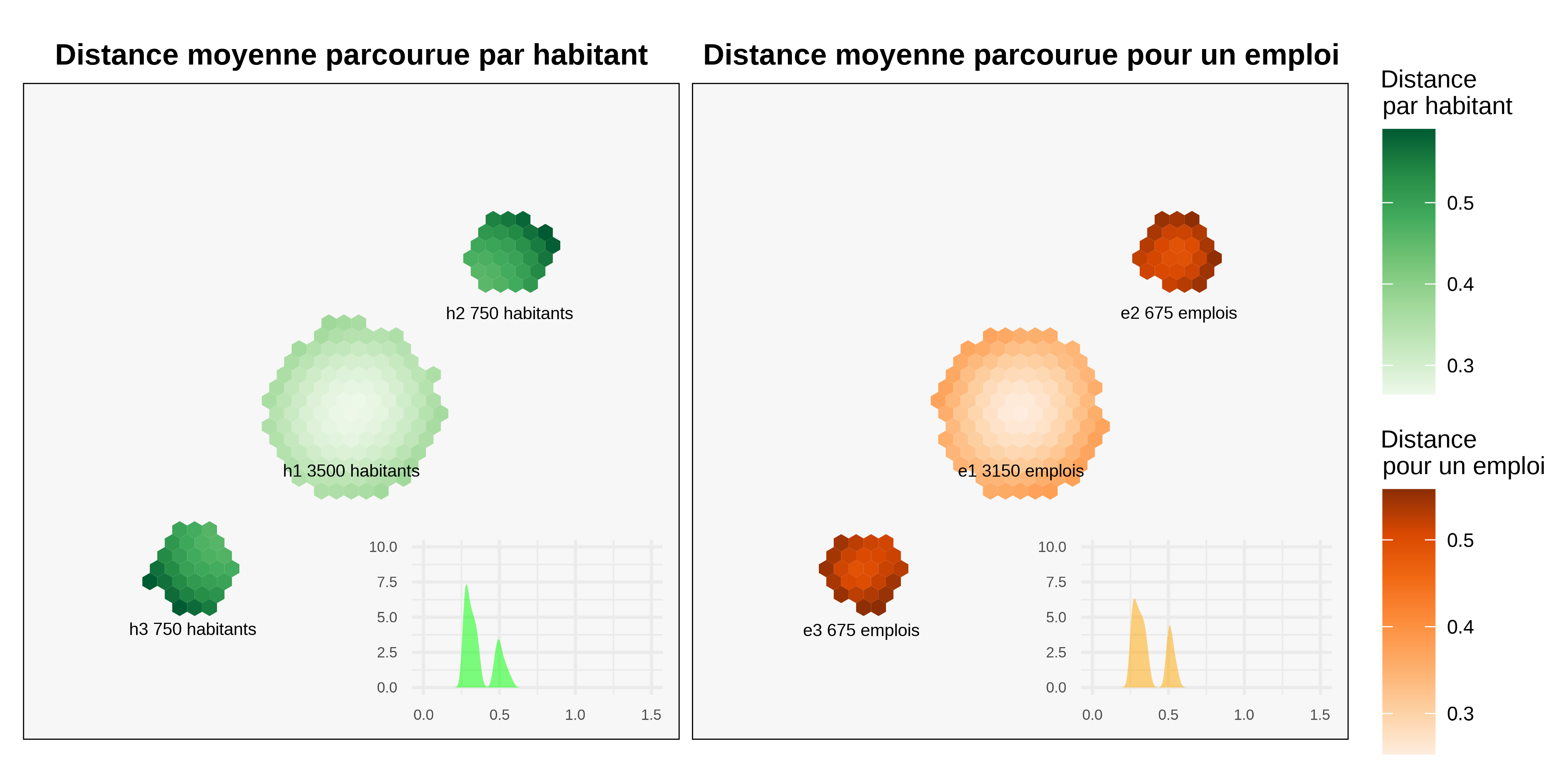
This first figure shows how the MEAPS model works. A distribution of journeys can be generated (in the small graphs of the figure 2). As the majority of jobs are located in the central hub, the average distances for residents are lower there than in the other hubs. The model generates a little variance within each centre. This is consistent with the idea that the most outlying residential hexagons generate greater distances. The distribution of average distances to employment is tighter than that of average distances travelled per inhabitant. The averages of these two distributions are equal (by design).
We can construct a table of flows between each centre (table 2). The first thing to note is that the constraints at the margins are perfectly respected, which is the principle behind the construction of MEAPS, the approximations made in the resolution algorithm thus remaining less than 10^{-5} at least. Furthermore, the table of flows confirms the previous assessment. Most of the residents of h1 (78%) move to g1 (the same centre). This “intra-cluster” employment rate is 42% for the other two clusters. This is due to the imbalance in the location of jobs and is a desired property of the model. It partly explains the distribution of job mobility distances for residents and also its ‘reciprocal’, when calculating average distances to a hexagon of jobs.
| e1 | e2 | e3 | total | |
|---|---|---|---|---|
| h1 | 2 481 | 335 | 334 | 3 150 |
| h2 | 334 | 290 | 51 | 675 |
| h3 | 334 | 50 | 290 | 675 |
| total | 3 150 | 675 | 675 | 4 500 |
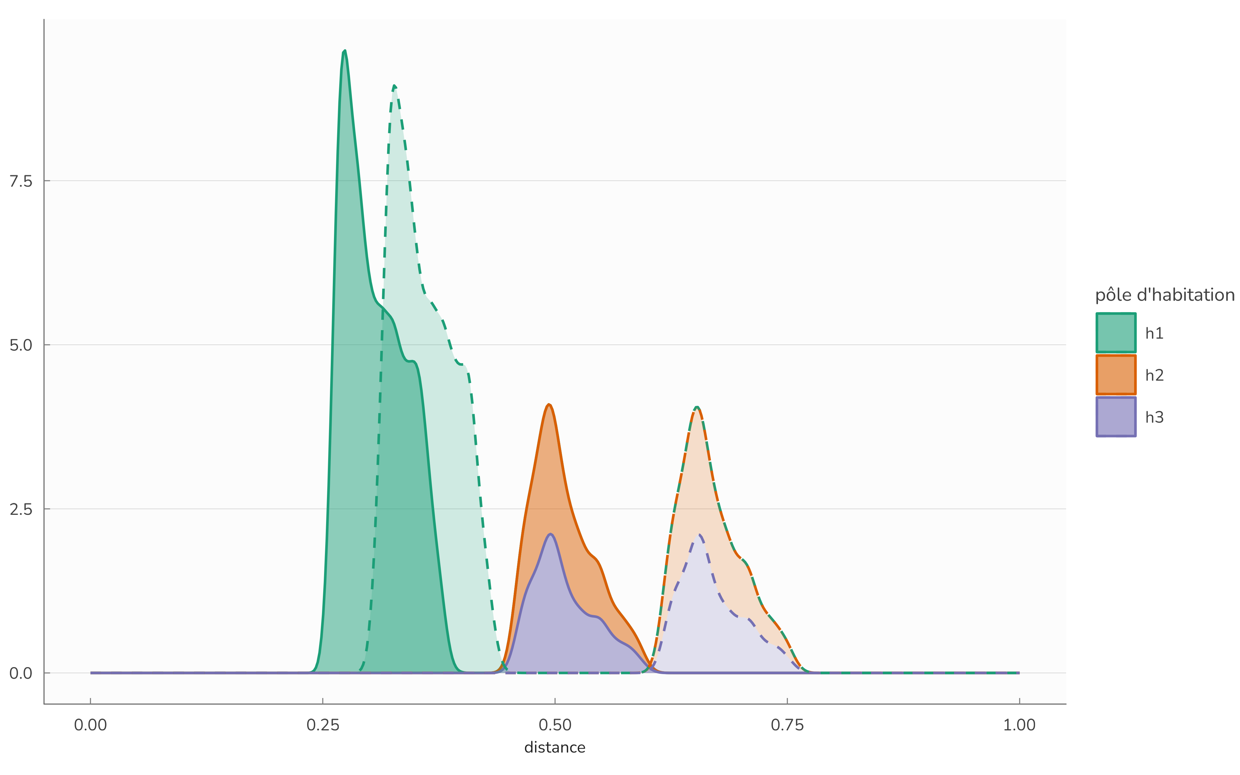
To assess the behaviour of the model, we can perform a thought experiment in which we move the two satellite poles away from the centre (the distance between 1 and 2 or 3 increases from 0.7 to 1.2 in this experiment). The table 3 is obtained by simulating the model again on this alternative geography. The result is identical to the previous configuration. This result is consistent with intuition and is a desired property of the model. Since the ranking orders do not change (as long as the poles are far enough apart and the configuration remains symmetrical), the ranks are not modified and therefore the flows are unchanged. The distributions of distances (outgoing and incoming) are largely modified, since 2 or 3 are further away from 1, as indicated by figure 3. We are tempted to conduct further thought experiments to analyse the behaviour of the model. The application Shiny application available at ofce.shinyapps.io/rmeaps allows all these experiments to be carried out using the same code as is used here.
| e1 | e2 | e3 | total | |
|---|---|---|---|---|
| h1 | 2 482 | 334 | 334 | 3 150 |
| h2 | 334 | 290 | 51 | 675 |
| h3 | 334 | 51 | 291 | 675 |
| total | 3 150 | 675 | 675 | 4 500 |

4.2 Comparison with the gravity model
Comparing MEAPS with the gravity model allows us to understand its advantages. To do this, we simulate a gravity model with two constraints equation 3, to allow calibration on the rows (each individual has a job) and on the columns (each job is filled). This model is simulated at the disaggregated level, i.e. at the level of each individual and each job based on the geographical configuration described above in section 4.1. The gravity model is specified using the functionf where \delta is a positive parameter :
f(d) = e^{d/\delta} \tag{22}
This is a very common choice for modeling of trip flows. The gravity model can then be normalised using the Furness algorithm (Dios Ortúzar & Willumsen, 2011), in which first the rows are normalised (each individual has one job and one job only in probability, taking into account the migration parameter), then the columns (each job is completely filled). These normalisations are iterated in rows and then in columns until a stable flow matrix is obtained. These normalisations follow the equation 4 and equation 5 normalisations.
The gravity model adapted in this way is fitted to the MEAPS simulation, taking as a reference the flows of table 2, constructed by aggregation over groups of inhabitants and jobs – in other words a matrix of 3 \times 3. The adjustment is made by calibrating the parameter \delta so as to minimise the relative Kullback-Leitner entropy of the aggregated distributions (this notion of entropy is described in detail in the document Estimates at La Rochelle). The result of the estimation is proposed in table 4 and corresponds to a value of \delta \approx 0.68.
| MEAPS Migration at 10% |
Gravitaire Adjusted, δ = 0.68 |
|||||||||
|---|---|---|---|---|---|---|---|---|---|---|
| e1 | e2 | e3 | total | e1 | e2 | e3 | total | |||
| h1 | 2 481 | 335 | 334 | 3 150 | h1 | 2 447 | 352 | 350 | 3 150 | |
| h2 | 334 | 290 | 51 | 675 | h2 | 353 | 286 | 36 | 675 | |
| h3 | 334 | 50 | 290 | 675 | h3 | 350 | 37 | 288 | 675 | |
| total | 3 150 | 675 | 675 | 4 500 | total | 3 150 | 675 | 675 | 4 500 | |
The adjustment of the gravity model gives a good result. One of the reasons for this good result is the symmetry of the geographical configuration. The two satellites are at the same distance from the central pole and the f function, which depends only on distance, ensures that the flows are distributed between each of the poles without too much difficulty. If we take a non-symmetrical configuration, by moving one of the two satellites further away, with the other remaining in its place, we obtain a different pattern, with the gravity model amplifying the asymmetries.
| MEAPS Migration at 10% |
Gravitaire Adjusted, δ = 0.68 |
|||||||||
|---|---|---|---|---|---|---|---|---|---|---|
| e1 | e2 | e3 | total | e1 | e2 | e3 | total | |||
| h1 | 2 482 | 334 | 334 | 3 150 | h1 | 2 581 | 285 | 284 | 3 150 | |
| h2 | 334 | 290 | 51 | 675 | h2 | 286 | 367 | 22 | 675 | |
| h3 | 334 | 51 | 291 | 675 | h3 | 284 | 23 | 369 | 675 | |
| total | 3 150 | 675 | 675 | 4 500 | total | 3 150 | 675 | 675 | 4 500 | |
The model MEAPS model maintains an identical configuration in the case of satellite centres that are far from the centre, because the configuration remains symmetrical and no rank is changed. On the other hand, the gravity model gives a very different response to that of the reference case: satellite residents are more inclined to look for jobs in their respective satellites, and the flows between satellite poles and the central pole are reduced. This property of the gravity model is expected: the function f function gives less weight to jobs that are further away. At the limit where this distance becomes particularly great, the flows between satellite centres and the central centre will dry up almost entirely. The estimated parameter for the MEAPS simulation is of the order of 0.68 which is of the order of magnitude of the radius of the central pole (0.5). For a distance of a few times 0.68 the flux between poles will be almost zero. MEAPS’ result seems more appropriate to the situation we are observing. When municipalities are satellites of a central hub at a distance of a few dozen kilometres, there are flows towards this municipality to take up jobs, and the fact that the municipality is a few kilometres further away does not drastically stop these flows. The sensitivity of distance is expected to be low at this scale. We will see when we apply this to the La Rochelle area, using data describing flows between the towns of residence and the towns of employment (taken from INSEE (2022)) that MEAPS provides a better representation of reality than the gravity model.
If we re- estimate the parameter \delta for the geographical configuration in which the satellite centres are far apart, we end up with \delta \approx 0.95. This value is very different from the previous parameter, which shows both the ‘plasticity’ of the gravity model and its unreliability, as if the ‘gravitational’ force could change completely with each new datum (table 6).
| MEAPS Migration at 10% |
Gravity Readjusted, δ = 0.95 |
|||||||||
|---|---|---|---|---|---|---|---|---|---|---|
| e1 | e2 | e3 | total | e1 | e2 | e3 | total | |||
| h1 | 2 482 | 334 | 334 | 3 150 | h1 | 2 455 | 348 | 347 | 3 150 | |
| h2 | 334 | 290 | 51 | 675 | h2 | 348 | 288 | 39 | 675 | |
| h3 | 334 | 51 | 291 | 675 | h3 | 347 | 39 | 289 | 675 | |
| total | 3 150 | 675 | 675 | 4 500 | total | 3 150 | 675 | 675 | 4 500 | |
4.3 Estimation procedure
It is possible to modify the weights of the absorption probabilities so as to adjust the table of rates of flux. This is illustrated in the following table, where for each of the 9 possible pairs of residential area (3) and employment area (3) the relative probability of absorption has been doubled, in succession. The geographical configuration is that of the figure 1, with a centre and two satellites. The centre contains more jobs than residents, forcing inflows into zone 1 as indicated in the table 2. This constitutes a relative doubling of the probability, because the constraints of a constant probability of migration and the saturation of jobs impose a reduction in the probability of absorption in other jobs, a key feature of the algorithm which implements MEAPS.
The table 7 illustrates the variations in fluxes compared with a reference situation (that of the table 2), rounded to the nearest integer. There are therefore 3 \times 3 matrices 3 \times 3. Each of the sub-matrices indicates the flux variations for each origin-destination pair; there are 9 possibilities for doubling the absorption probability, which constitute the rows and columns of the encompassing matrix. Note that the sums of the columns and rows of each sub-matrix are zero, indicating that the row and column constraints have been met.
Intuition would imply that the residential/employment zone pair, which is increased in relative probability, would experience higher flux. Indeed, this increase of flux is observed in the results, despite the effects induced by compliance with the row and column constraints. To compensate for these higher rates of flux, in the same column, i.e. for flows from other residential areas, there is a systematic decrease in fluxes from other residential areas. Symmetrically, an increase in flows from the residential area i to the employment zone j always leads to a decrease in flows from i to other employment areas.
| e1 | e2 | e3 | ||||||||
|---|---|---|---|---|---|---|---|---|---|---|
| e1 | e2 | e3 | e1 | e2 | e3 | e1 | e2 | e3 | ||
| h1 | h1 | 76 | −38 | −38 | −72 | 55 | 17 | −72 | 17 | 55 |
| h2 | −38 | 27 | 11 | 81 | −63 | −18 | −9 | 1 | 8 | |
| h3 | −38 | 11 | 27 | −9 | 8 | 1 | 81 | −18 | −63 | |
| h2 | h1 | −59 | 75 | −15 | 75 | −76 | 1 | 2 | −26 | 24 |
| h2 | 51 | −58 | 7 | −80 | 87 | −7 | 7 | −13 | 5 | |
| h3 | 9 | −17 | 8 | 5 | −11 | 7 | −9 | 39 | −30 | |
| h3 | h1 | −59 | −15 | 75 | 2 | 24 | −26 | 75 | 0 | −76 |
| h2 | 9 | 8 | −17 | −9 | −30 | 39 | 5 | 7 | −12 | |
| h3 | 51 | 7 | −58 | 7 | 5 | −12 | −80 | −7 | 87 | |
| The table represents the gap between the resulting flows for a doubled probability of absorption, for the residential zone i and the employment zone j, for each pair of residential/ employment zones. The first matrice at top left indicates that the flow between residential zone 1 and employment zone 1 is increased by 76 when the probability of relative absorption is doubled. To compensate these greater flows between zones 1 and 1, the flows between residential zone 2 and employment zone 1 are reduced by 38, which itself implies that those between 2 and 2 and between 2 and 3 are larger. | ||||||||||
An interesting property of the table 7 matrices is that the nine matrices 3 \times 3 form a vector space 11 of dimension 4. This is to be expected, as the constraints reduce the dimension by 9 (=3\times 3) to 4, since there are three constraints in each dimension (rows and columns) and one is redundant (if the sums on each row are zero, then the sum of all the coefficients is zero and therefore if the sums on two columns are zero, the third is necessarily zero). This indicates that, at least locally (in the vicinity of the flux matrix calculated in table 2), it is possible to modify the absorptional probabilities to achieve any matrix of flows. To the nearest linear approximation, it is therefore possible to reproduce any aggregate flow structure using a set of parameters that exactly saturate the dimension of this flow structure. This property means that different estimation approaches can be imagined, depending on the data available and the number of degrees of freedom we are prepared to commit to reproducing the data.
11 The eigenvalues of the 9 \times 9 consisting of the nine column vectors of the nine “derived” matrices are (133.3, 97.3, -28.6, 22.0, 0, 0, 0, 0, 0). With 5 zero eigenvalues and 4 non-zero eigenvalues, we can conclude that the dimension of the vector space generated by the nine matrices is 4.
The calculation time can be quite long due to the need to repeat a large number of draws, but the following section (section 4.4) shows that this number can remain reasonable. An estimate of this type is implemented by an iterative procedure in the document Estimates at La Rochelle document, which reproduces MEAPS data using the INSEE (2022) job mobility survey with a calculation scheme that can be easily implemented.
4.4 Ergodicity in practice
Using simulated data, it is straightforward to test the ergodicity hypothesis. This hypothesis conjectures that the mean values over u permutations are comparable to observations, ultimately repeated. At this stage of hypothetical simulations we do not compare the model with observations (see Estimates at La Rochelle), but we will show that estimating mean values does not require examination of the I! possible permutations 12 and can be accomplished with spatial aggregation and a limited number of permutation resamples.
12 By Stirling’s formula log_{10}(I!) \approx (n +1/2)log_{10} n +log_{10}\sqrt{2} - n log_{10}e \approx 5\times10^5 for I=10^5 which makes a large number.
To illustrate this property, we repeat the simulations of the model for several resamples of priority (noted u in the section 3.3 section), using a Monte-Carlo method. Taking the average over a sample of u we can construct an estimator of the mean values and show that with a sample size that is small compared with I!, the means can be estimated reliably and in a reasonable time. This property will be demonstrated on the particular geographical structure that we have simulated, although this does not allow us to generalise with certainty. There are undoubtedly aberrant spatial configurations that contradict this conjecture.
The figure 5 illustrates the stochastic processes at work in the model and their resolution by averaging over the possible resamples. The model is applied by randomly drawing permutations of different priority between residents. For several residential hexagons (randomly selected), we then identify the total set of destination choices (grouped within the hexagons). The grid already performs an averaging operation, since each individual in each hexagon has a different order of priority. We then represent the quantities of jobs (the probability of choosing a job in the destination hexagon). The white lines illustrate the dependence on the priority draw. But after a few draws, these probabilities converge on average. To simulate the model, it is not necessary (in all likelihood) to go through the entire universe of permutations.

The table 8 indicates confidence intervals of 90% that can be constructed from the previous simulations. Satisfactory stability is achieved, even though the aggregate flows are stochastic. For a hundred or so runs, we can obtain an accuracy of more than 10^{-3}.
| e1 | e2 | e3 | |
|---|---|---|---|
| h1 | 2481 |
335 |
334 |
| h2 | 334 |
290 |
51 |
| h3 | 334 |
50 |
290 |
| Source: MEAPS, interval at 95%, 1024 draws | |||
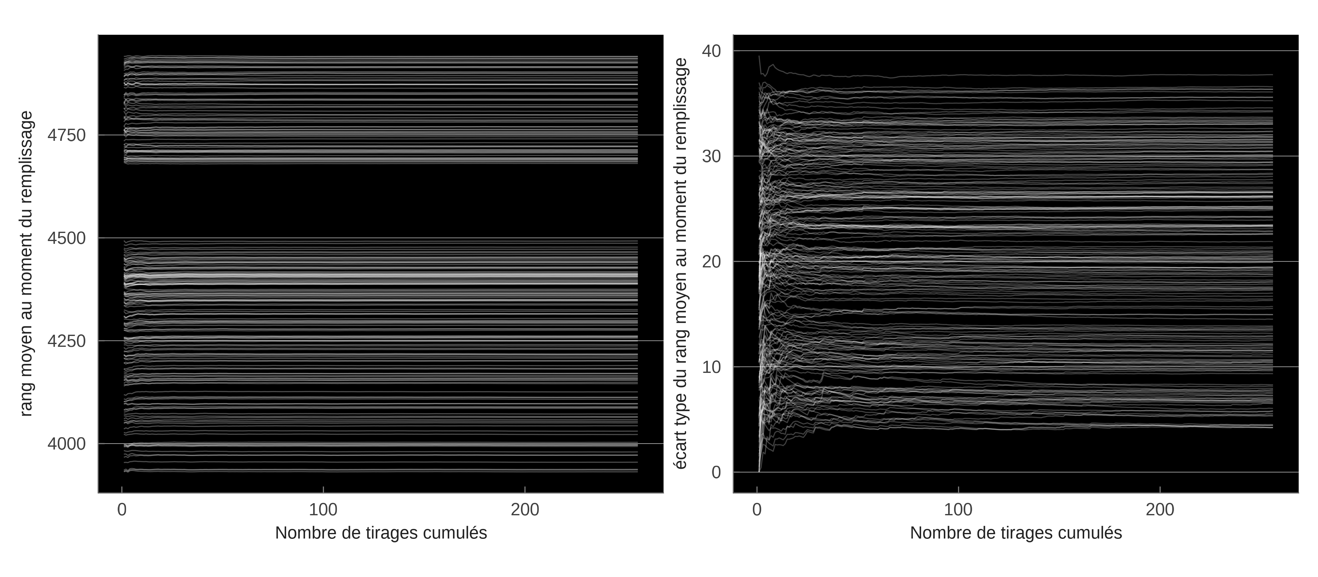
The saturation and priority diagram is illustrated by figure 6 below. For each destination square (a job), we represent the average rank (left) and its standard deviation (right) at the time of saturation. The stochastic nature results from the random drawing of the order of each individual (the starting squares). For most jobs, the mean ergodic saturation rank is reached very quickly. The white lines are rapidly horizontal, indicating rapid convergence of the mean rank as the draws accumulate. This graph confirms that, with a few exceptions, the state of the system is stable after a few draws. The right-hand panel illustrates the standard deviation observed on the cumulative draws. This illustrates the stochastic nature of the model induced by the draws.
4.5 Localised tension by job
The average rank at the time of saturation is information that can be used to construct a localised tension indicator as shown on figure 7. The tension indicator provides information that is distinct from average distance or population or job density. The most strained jobs are found on the axis linking the centres. Jobs located on the periphery of the central hub have a level of tension close to (but slightly higher than) those located in the satellites on the edge closest to the central hub. These factors can be used to identify relevant areas for employment development.
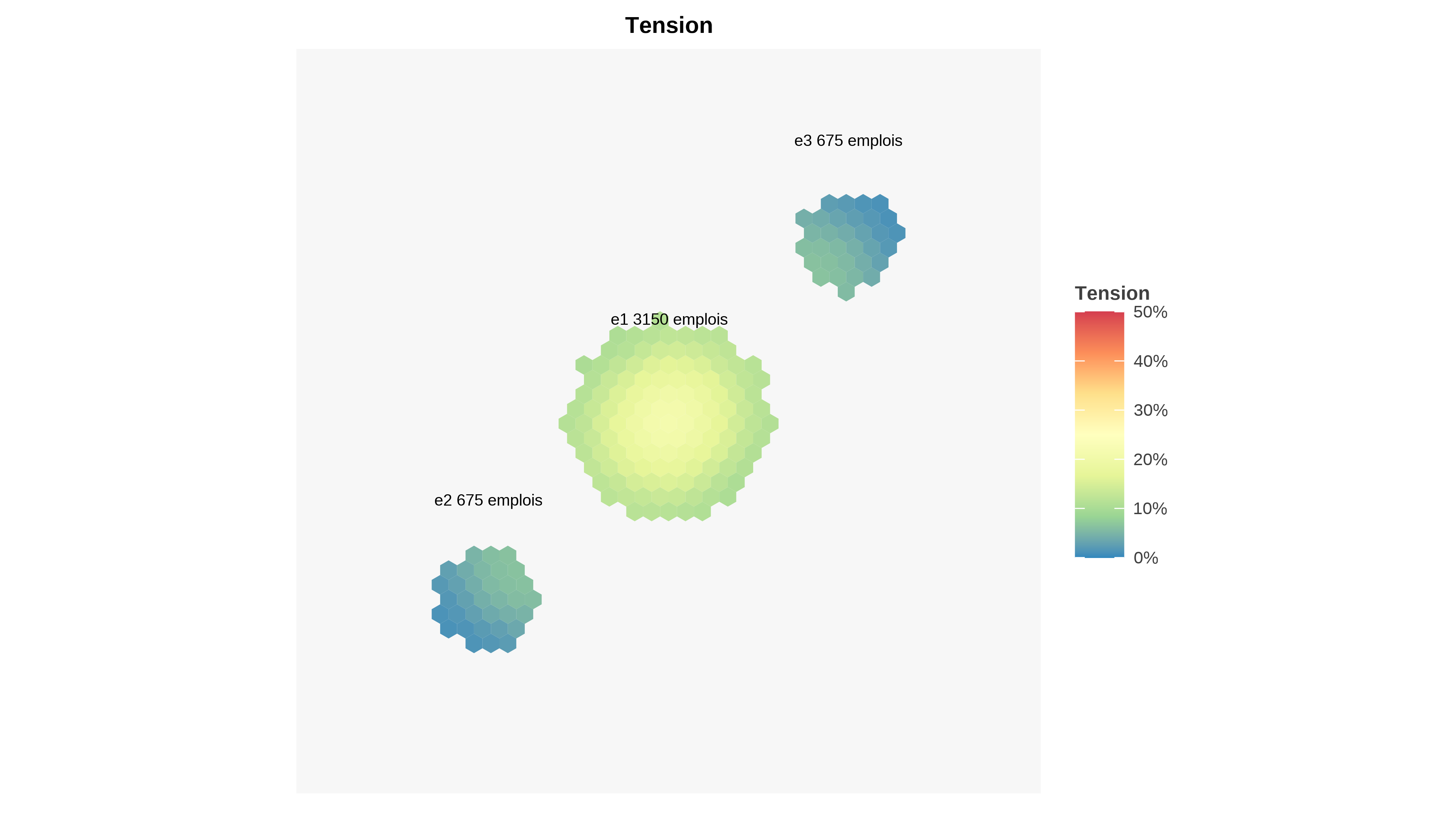
Experimentation in the application Shiny application makes it possible to study various properties of the tension indicator, in particular when overall tension is high (fewer jobs than residents) or low (excess of jobs over residents). In the case where there is an excess of jobs over residents, it is possible to observe local tension on certain jobs.
4.6 Synthetic simulation in Shiny
The application shiny rmeaps application can be used to generate hypothetical geographies and simulate the MEAPS model on these distributions. Most of the graphs in this chapter can be reproduced in this way. The application allows you to choose the size of the simulation (n the number of workers and k the number of jobs). By choosing more jobs than workers, we introduce a problem where there is an excess of jobs and therefore no migration constraint. In the opposite case, there is migration, calculated so that the number of working people remaining in the area is equal to the number of jobs.
Various parameters can be used to specify the geography, i.e. the relative position of the poles or their size. The simulator uses Monte Carlo to simulate several orders of passage and displays the corresponding graphs as convergence progresses, accumulating the average of the different variables in the model. This feature makes it easy to visualise the ergodicity property mentioned above.
References
Ben-Akiva, M., & Lerman, S. R. (2018). Discrete choice analysis: Theory and application to travel demand. MIT Press.
Commenges, H. (2016). Modèle de radiation et modèle gravitaire - Du formalisme à l’usage. Revue Internationale de Géomatique, 26(1), 79–95. https://doi.org/10.3166/RIG.26.79-95
Dios Ortúzar, J. de, & Willumsen, L. G. (2011). Modelling transport. John wiley & sons.
Fik, T. J., & Mulligan, G. F. (1990). Spatial Flows and Competing Central Places: Towards a General Theory of Hierarchical Interaction. Environment and Planning A: Economy and Space, 22(4), 527–549. https://doi.org/10.1068/a220527
Floch, J.-M., & Sillard, P. (2019). Les interactions spatiales. Quelques conséquences de l’introduction du modèle radiatif. Colloque Théo Quant 2019. Retrieved from https://thema.univ-fcomte.fr/theoq/pdf/2019/communications/2019_Floch.pdf
Fotheringham, A. S. (1983). A New Set of Spatial-Interaction Models: The Theory of Competing Destinations. Environment and Planning A: Economy and Space, 15(1), 15–36. https://doi.org/10.1177/0308518X8301500103
Fotheringham, A. S. (1984). Spatial Flows and Spatial Patterns. Environment and Planning A: Economy and Space, 16(4), 529–543. https://doi.org/10.1068/a160529
Hansen, W. G. (1959). How accessibility shapes land use. Journal of the American Institute of Planners, 25(2), 73–76. https://doi.org/10.1080/01944365908978307
Heanue, K. E., & Pyers, C. E. (1966). A comparative evaluation of trip distribution procedures. Highway Reserach Record, (114), 20–50.
INSEE. (2022). Mobilités professionnelles en 2019 : Déplacements domicile - lieu de travail recensement de la population - base flux de mobilité [Data set]. INSEE. Retrieved from https://www.insee.fr/fr/statistiques/6454112
Koenig, G. (1980). Indicators of urban accessibility: Theory and application. Transportation, 9(2), 145–172. https://doi.org/10.1007/bf00167128
Lasser, J. (2020). Creating an executable paper is a journey through Open Science. Communications Physics, 3(1). https://doi.org/10.1038/s42005-020-00403-4
Lenormand, M., Bassolas, A., & Ramasco, J. J. (2016). Systematic comparison of trip distribution laws and models. Journal of Transport Geography, 51, 158–169. https://doi.org/10.1016/j.jtrangeo.2015.12.008
Masucci, A. P., Serras, J., Johansson, A., & Batty, M. (2013). Gravity versus radiation models: On the importance of scale and heterogeneity in commuting flows. Physical Review E, 88(2), 022812. https://doi.org/10.1103/PhysRevE.88.022812
McFadden, D. (1974). The measurement of urban travel demand. Journal of Public Economics, 3(4), 303–328. https://doi.org/10.1016/0047-2727(74)90003-6
Parodi, M., & Timbeau, X. (2024a). La ville compacte : Une solution aux émissions de gaz à effet de serre. Document de Travail de l’OFCE, (5-2024). Retrieved from https://preview.meaps.fr/trajets.html
Parodi, M., & Timbeau, X. (2024b). MEAPS&gravitaire : Estimations à la rochelle. Document de Travail de l’OFCE, (4-2024). Retrieved from https://preview.meaps.fr/larochelle.html
Patrick Bonnel. (2001). Prévision de la demande de transport (PhD thesis). Lyon, France.
Ruiter, E. R. (1967). Toward a better understanding of the intervening opportunities model. Transportation Research, 1(1), 47–56. https://doi.org/https://doi.org/10.1016/0041-1647(67)90094-9
Sen, A., & Smith, T. E. (1995). Gravity models of spatial interaction behavior. Berlin, Heidelberg: Springer. https://doi.org/10.1007/978-3-642-79880-1
Simini, F., González, M. C., Maritan, A., & Barabási, A.-L. (2012). A universal model for mobility and migration patterns. Nature, 484(7392), 96–100. https://doi.org/10.1038/nature10856
Simini, F., Maritan, A., & Néda, Z. (2013). Human Mobility in a Continuum Approach. PLOS ONE, 8(3), e60069. https://doi.org/10.1371/journal.pone.0060069
Stouffer, S. A. (1940). Intervening opportunities: A theory relating mobility and distance. American Sociological Review, 5(6), 845. https://doi.org/10.2307/2084520
Wilson, A. G. (1967). A statistical theory of spatial distribution models. Transportation Research, 1(3), 253–269. https://doi.org/10.1016/0041-1647(67)90035-4
Reuse
Citation
BibTeX citation:
@article{parodi2023,
  author = {Parodi, Maxime and Timbeau, Xavier},
  title = {MEAPS: {Modelling} Commuter Flows {\^{}{[}Translation} by
    {Scotia} {Hille{]}}},
  journal = {OFCE Working Paper n°2023-15},
  date = {2023-05-02},
  url = {https://preview.meaps.fr},
  langid = {en},
  abstract = {The gravity model used to distribute journeys between an
    origin and a destination poorly represents the influence of distance
    on choices. Drawing on the “intervening opportunities” model of
    @stouffer1940 and the radiative model of @simini2012, we construct
    an ergodic model of absorption with priority and saturation (MEAPS)
    that makes it possible to construct these choices on clear and
    flexible microscopic foundations. The model accommodates different
    formulations of stochastic processes that allow fundamental
    parameters to be estimated and interpreted. We validate the
    theoretical model on synthetic data, then in two associated
    documents {[}@meaps2024a; @meaps2024b{]} We propose an estimate of
    MEAPS and a detailed comparison with the gravity model and its most
    common variants. We then use this modelling to construct a
    high-resolution map of CO\textasciitilde2\textasciitilde{} emissions
    in La Rochelle. \textless br\textgreater{} `r
    wordcountaddin::word\_count(“theorie.en.qmd”)` words.}
}
For attribution, please cite this work as:
Parodi, M., & Timbeau, X. (2023). MEAPS: Modelling commuter flows
^[Translation by Scotia Hille]. OFCE Working Paper n°2023-15.
Retrieved from https://preview.meaps.fr